Growth Rate Forecast
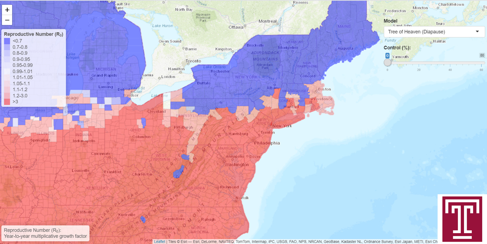
Description: Maps of the one-year temperature-dependent reproductive number (R0)–that is, the factor by which the population grows (or decreases) in one year–assuming feeding on different host plants, the possibility or lack of diapause, and varying levels of control. (Also termed “(net) reproductive rate”.) Calculated with a stage-age-structured system of partial differential equations based on calibrated parameters of SLF biology and temperature sensitivity.
How to Use the App: Use the drop-down menu in the upper right corner to select a host plant (tree of heaven or maple) and diapause assumption (diapause or non-diapause). (Note: If diapause is selected, all eggs laid in the summer and fall pass through diapause, while those laid in the winter and spring do not. If non-diapause is selected, no eggs are ever laid in diapause.) The menu option “difference” displays a map of the difference in R0 under the tree of heaven and maple models. Use the slider below the drop-down menu to see how R0 changes when the level of control is varied. (Note: Here, “control (%)” is the fraction of the egg population that is killed by control measures.)
Interpretation: Predictions of the annual R0 based on annual temperature profiles and parameters of SLF biology and temperature sensitivity.
Accuracy: Results based on mean temperatures (2010-2018); may not reflect extreme temperature anomalies.
Assumptions:Results are based on daily mean temperatures averaged over eight years (2010-2018) and thus represent R0 values expected under average conditions. May fail to represent R0 accurately during years with very anomalous temperature patterns (e.g., extreme heat waves or cold spells, etc.). Does not take into account other effects of climate, like soil moisture.
Citation: Lewkiewicz S M, De Bona S, Helmus M R, Seibold B. 2022. Temperature sensitivity of pest reproductive numbers in age-structured PDE models, with a focus on the invasive spotted lanternfly. Journal of Mathematical Biology. 85(3): 1-37. doi.org/10.1007/s00285-022-01800-9
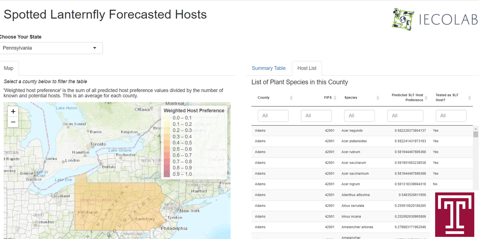
Description: This app provides forecasted plant hosts for SLF that are organized by US state and counties within states. To predict host preference, we used known SLF host records obtained from the literature (primarily from Barringer & Ciafré 2020, doi:10.1093/ee/nvaa093) and phylogenetic relationships among vascular plant species (built with the R package V.PhyloMaker; see Jin & Qian 2019, doi:10.1111/ecog.04434). We implemented Hidden State Prediction (HSP; see Zaneveld & Thurber 2014, doi:10.3389/fmicb.2014.00431) with the plant host phylogeny to predict a binary response of either adult or nymph and adult use. HSP is methodologically similar to ancestral state reconstruction but more flexibly allows for prediction of unknown tip states in the phylogeny (not just internal nodes). For our analyses, we elected to use a fixed-rates continuous-time Markov model implementation of HSP to allow for maximum likelihood estimation of model parameters. HSP produces likelihood estimates for each possible state, and we report the likelihood of SLF using each tree species as a host either as an adult or nymph and adult. We intersected these predicted feeding preference values with county level inventories of plant species by US state and county (obtained and cleaned from the PLANTS database, http://plants.usda.gov). The resulting county level data were summarized and weighted for comparison as the sum of preference values for a county divided by the number of unique species in that county.
How to Use the App: The interface of this app contains two main sections: (1) a county level map of US states that contains weighted host preference for each county and (2) a dynamic summary table of host preferences for that state and county. To switch between states, select your choice with the ‘Select State’ dropdown menu. Map navigation follows the typical controls for online map apps: drag to move location and zoom in or out with the plus and minus symbols in the upper left map corner. The table has two tabs, ‘Summary Table’ and ‘Host List’. Summary Table contains county level host preference data that link directly to the current map selection, including identifying county information, number of known and potential tree host species, and the weighted host preference. Host List contains the same county information, the latin name of each species, its SLF preference (‘Predicted Preference’), and whether or not that host is a previously known host or a predicted tree host (‘Host Status’). Both tables can be sorted by selecting the column headers or filtered by entering filter criteria in the bar at the top of each column header. Notably, selecting a county on the map will filter the tables to display corresponding county data and filtered species list, but if no county has been selected for a state, data for all counties in a state are shown. To return to all counties within the selected state, simply click any location on the map outside the state boundaries
Interpretation: This app can be used to identify areas (counties within a state) that may have a large number of plant species that may be suitable hosts for SLF. Lists of known or potential plant hosts serve as a guide of species to monitor for SLF and impact. The data reported here should be treated as predictions of SLF preference that are subject to new data updates, except where known hosts are reported.
Accuracy: This app contains preliminary data from ongoing analyses. The forecasted hosts do not include model testing of known hosts (e.g., crossvalidation), but further model evaluation is ongoing. Caution should be applied to predictions made in the current version of the app.
Assumptions: Feeding preference is assumed to have a strong and consistent phylogenetic signal, indicating that closely related species are likely to be preferred at similar levels by SLF. Furthermore, this approach relies on sufficient sampling for known hosts (or not hosts), which may lead to poor predictive ability of our model if data are limited. The known preference data here are coarse in interpretation, as we use a binary variable of known preference that only considers adult or nymph and adult host use. Lastly, we consider only potential hosts that are considered tree species, but known hosts fall outside these categories. It is likely that some other non-tree species may be likely hosts as well but fall outside the current scope of the app. This app will be updated as additional data become available.
Citation: Huron, N. A. & Helmus, M. R. Predicting host preference and impact of spotted lanternfly on trees across the USA. in prep.

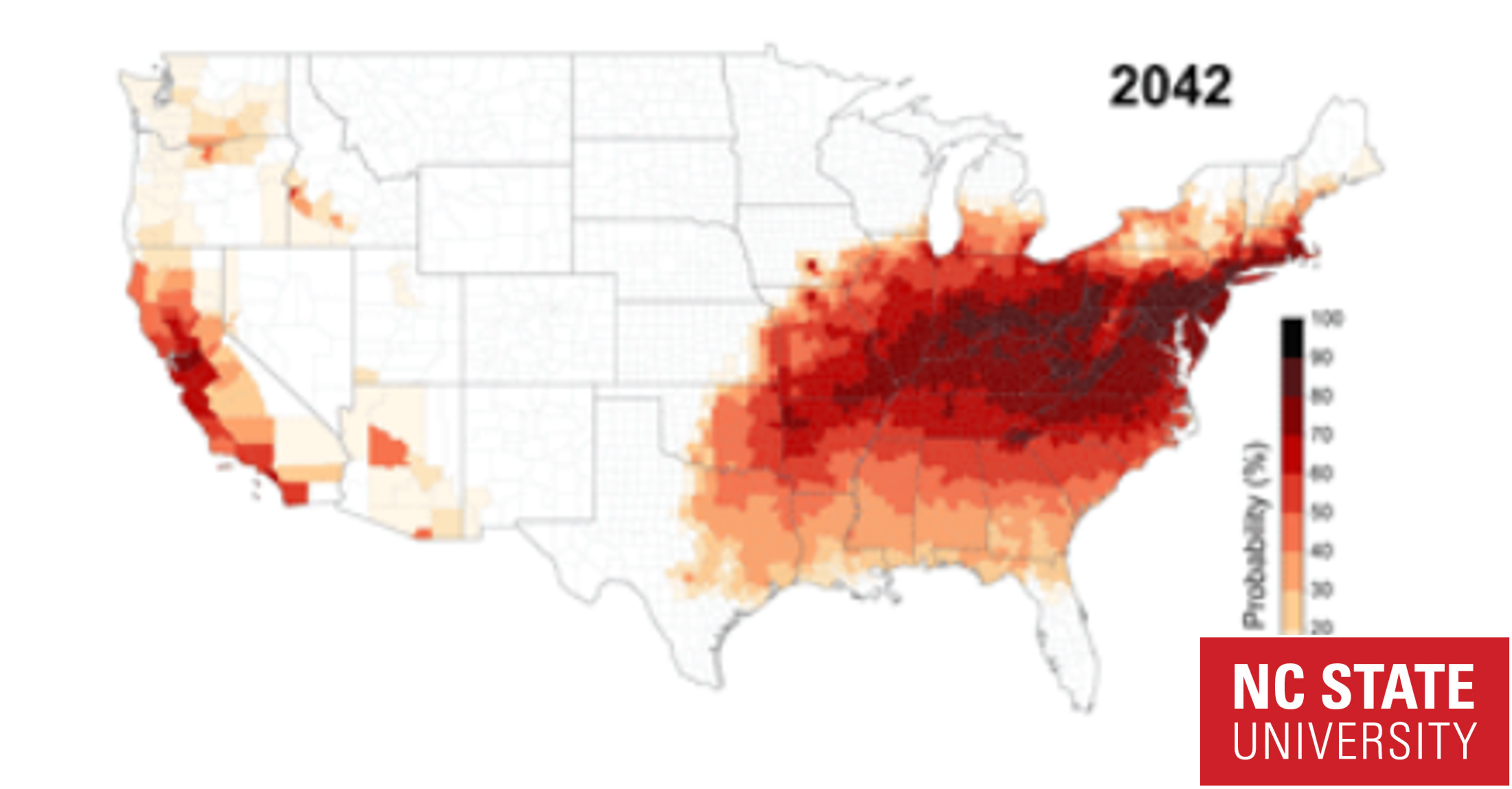
Description: The app shows the forecasted spread of SLF, at the county level, according to the predictions generated by a Generalized Dispersal Kernel model. This is a general, top-down model that uses past data on presence/absence of SLF to parameterize a dispersal kernel, used to predict future spread. Dispersal depends on generic drivers, such as human population density, forest cover, and tree density. The parameters of the model are validated using the presence/absence data from the latest year on record, and the model is then used to forecast SLF spread. The app shows the estimated spread risk, expressed in predicted years since establishment at the county level.
How to Use the App: The user can press the “play” button on the top-left corner to visualize the forecasts through time, or hand select a specific year using the slider.
Interpretation: The app shows forecasts representing a predicted future risk.
Accuracy: These forecasts are generated using a generic model of dispersal, and therefore have low accuracy, especially over long timespans. The model parameters are calibrated to SLF, but the drivers itself are generic and derived from a meta-analysis of other invasive forest pest species.
Assumptions: The model makes simplifying assumptions regarding the biology of the study species. Population growth rate is assumed to be homogeneous through space, therefore excluding the effect of climate on establishment potential and population growth. Host presence is interpreted in a generic sense, and depends on forest cover and tree density. Dispersal between two counties is calculated in relation to host presence and human population density in both origin and destination, to account for human-assisted transport.
Citation: Huron, N. A. & Helmus, M. R. Predicting host preference and impact of spotted lanternfly on trees across the USA. in prep.
Hudgins EJ, Liebhold AM, Leung B. 2017. Predicting the spread of all invasive forest pests in the United States. Ecology Letters 20: 426–435.
Hudgins EJ, Liebhold AM, Leung B. 2020. Comparing generalized and customized spread models for nonnative forest pests. Ecological Applications 30(1): e01988.
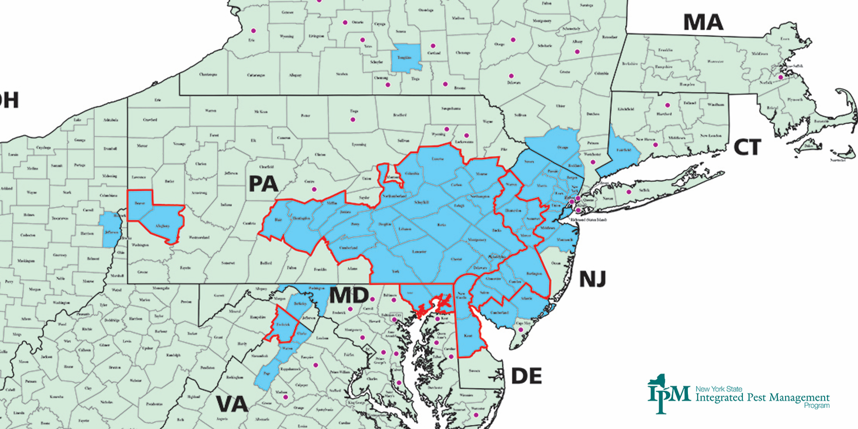
Description: Click on the app for more information.
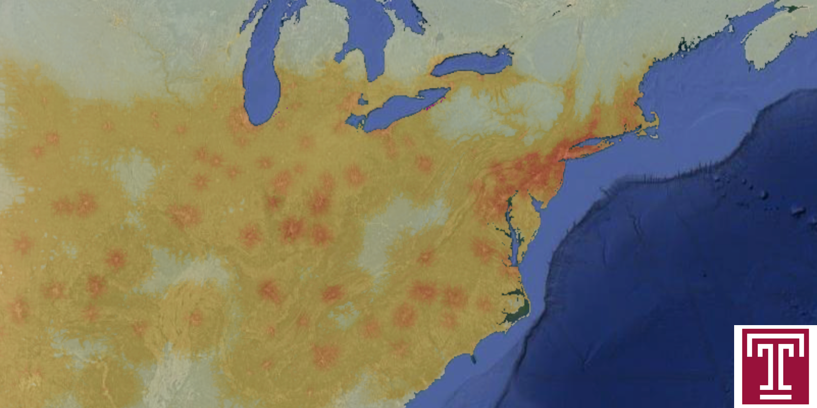
Description: Click on the app to view more information on their website.
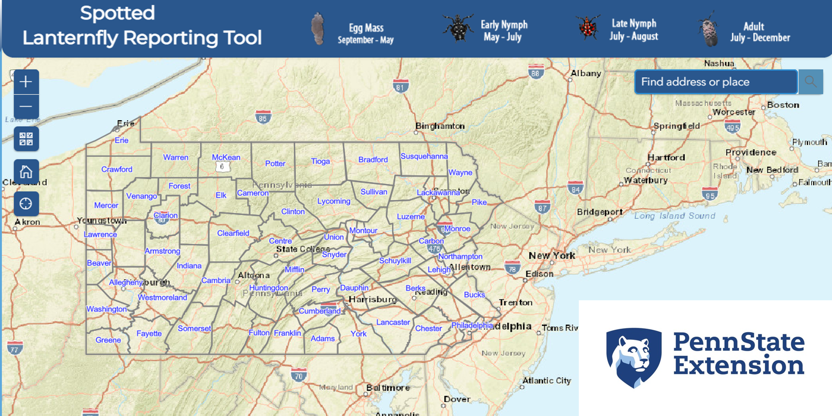
Description: Click on the app to view more information on their website.
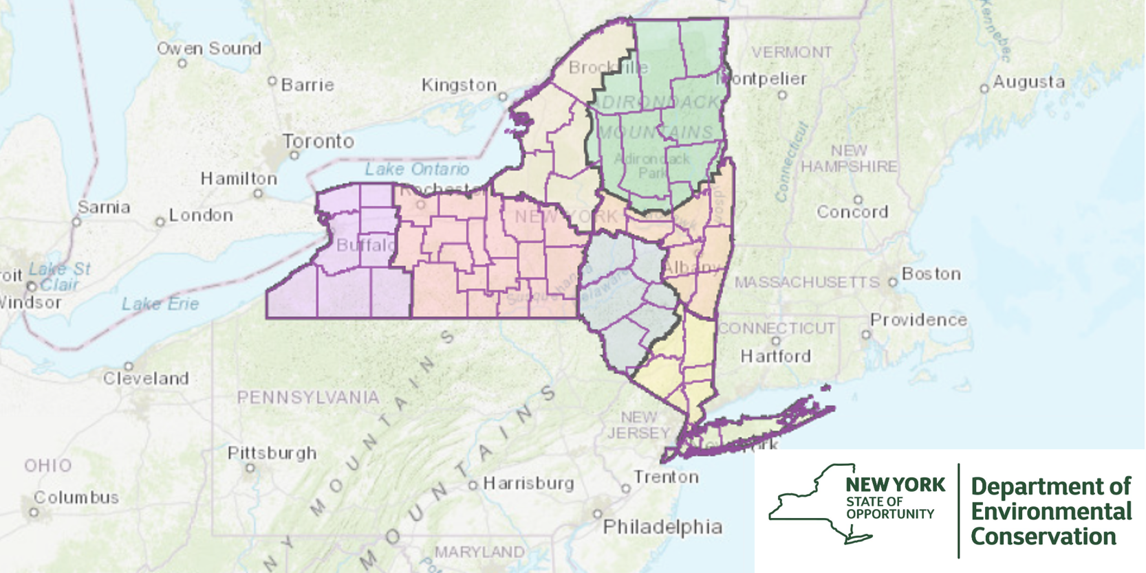
Description: Click on the app to view more information on their website.
Description: Click on the app to view more information on their website.
Description: Click on the app to view more information on their website.

Description: This R package combines survey datasets produced by different agencies (at the local, state, and federal level) in the United States into an aggregated and anonymized data set. This dataset includes information on approximate locations where each survey was conducted, the provenance of the data point, and the biologically relevant results of the surveys (presence/absence of SLF, presence of an established SLF population, and estimated population density of this pest).
How to Use the App: Users can see the R package documentation to see detailed ways on how to obtain the package and data associated with it.
Interpretation: The displayed information comes from survey data collected by local, state, and federal level agencies.
Accuracy: The data is aggregated from multiple sources and therefore has high degree of trust.
Assumptions:The density values for each county/10km grid cell are attributed as the highest density recorded in the area (county or grid cell) in a given year. Regulatory incidents are derived from data and personal communication.
Citation:De Bona, S., L. Barringer, P. Kurtz, J. Losiewicz, G.R. Parra, & M.R. Helmus. lydemapr: an R package to track the spread of the invasive spotted lanternfly (Lycorma delicatula, White 1845) (Hemiptera, Fulgoridae) in the United States. NeoBiota 86: 151-168. https://doi.org/10.3897/neobiota.86.101471

Description: This map shows the timeseries of past spread of SLF since its introduction in Berks County, PA. The spread is shown both at the county level and at a higher spatial resolution of 10km2. The user can toggle between maps showing how population density of established SLF populations changed through time (county-level and 10km2-level), and a map of regulatory incidents (county level-only), including counties where SLF was accidentally transported without leading to establishment.
How to Use the App: Use the dropdown menu on the top right corner to toggle between density maps (county-level and 10km2-level) and regulatory incident maps. The slider allows the user to either pick a specific year (by dragging it sideways) or display the spread through time by hitting the “play” button.
Interpretation: The displayed information comes from survey data collected by state and federal agencies.
Accuracy: The data is aggregated from multiple sources and therefore has high degree of trust.
Assumptions:The density values for each county/10km grid cell are attributed as the highest density recorded in the area (county or grid cell) in a given year. Regulatory incidents are derived from data and personal communication.
Citation:De Bona S, Hudgins E, Helmus M. A framework to document and forecast the spread of recent invasive species and its application to the Spotted Lanternfly. In prep.

Description: Jump dispersal is responsible for SLF establishment in distant, uninvaded regions as a result of human-assisted dispersal. This app provides standardized risk estimates of SLF jump dispersal and survey priority for 16 property types, including transport infrastructures. Jumps were identified every year as any established SLF population situated > 15 km from other SLF populations and any past jump dispersal, based on past spatial occurrence data (see Past Spread– Interactive Map). The observed distance between past jumps and each property type was compared to simulated averages (10,000 datasets of random points within the convex hull of the positive surveys). The standardized risk estimates are the effect size of the difference between observed and simulated data: the higher the standardized risk estimate for a given property type, the closer jumps were found from this property type compared to random simulations. Survey priorities were established as the inverse proportion of the standardized risk estimates.
How to Use the App: A table- Columns provide standardized risk estimates, survey priority and a description of property types included. A figure- standardized risk estimate per property type.
Interpretation: Future jumps are likely to occur at categories of properties with high survey priority. SLF surveys in uninvaded regions should focus primarily on properties ranked with high priority, as they are the most likely to be subject to jump dispersal, for an early detection of SLF jumps, which in turn maximizes the effectiveness of eradication and control measures.
Accuracy: Confidence in the survey priorities is high thanks to statistical evidence from models on the proximity between jumps and property types.
Assumptions:Jumps are found close to landscape features that facilitate their spread. The location of jumps that occurred up until 2020 is representative of future jump locations.
Citation:Belouard N., De Bona S., Helmus M.R., Behm J.E. Identify and predict jump dispersal in recent biological invasions based on spatial occurrence data. In prep.
Description: This app provides a map of invasion potentials for a paninvasion of SLF to impact the global wine market. Transport, establishment, and impact potentials are estimated for each country (all but impact potential are also shown for each US state). Transport potential is estimated as the average annual metric tonnage of trade with US states that are considered to have established SLF populations for 2012–2017. Establishment potential is the maximum predicted suitability for SLF within an area from an ensemble of species distribution models for SLF (see citation and compendium for further details on modeling methods). Impact potential is the average annual production tonnage of grapes for a region for 2012–2017. Notably, impact potential is not present in the app, which instead includes invasion risk for countries without established SLF. Invasion risk is calculated as the predicted impact potential (rescaled 1–10) from multivariate regression of impact potential (grape production) on transport and establishment potential.
How to Use the App: Please see the slfrsk research compendium vignette website for more information on how to use this app.
Interpretation: Areas that contain high values for invasion risk (thus all invasion potentials) suggest that there is a high risk of SLF getting transported from the US invaded region, establishing a population, and impacting the wine market for that region. Such areas should be considered at great risk and should be prioritized for monitoring and control efforts if SLF is found there. Regions where both transport and establishment potential are both high should also be considered high priority regions for monitoring spread. The values reported in this app should be seen as potentials to monitor as they become realized.
Accuracy: Given the multitude of data sources in this app, values reported within it should be treated as estimates that are likely to change as additional data become available. However, invasion potentials used in this app appear to correspond well with other analyses. Transport potential is correlated with known US states with established SLF as well as documented regulatory events (see citation supplementary information for further detail). Similarly, the establishment potential used here is extracted from an ensemble of species distribution models that appears to correspond with existing suitability models (both correlative and mechanistic). Lastly, despite the intricacies of grape cultivation vs. wine production for individual countries and US states, we find that either measure of impact appears to correlate with the other two invasion potentials, indicating strong confidence in the overall invasion risk for countries in the app.
Assumptions:Given the predictive nature of this app, all invasion potentials used can be considered estimates of empirical probability of transport, establishment, and impact of SLF from the US invaded region. The citation included below contains a caveats section that more explicitly details important assumptions that also pertain to this app.
Citation:Huron, N. A., Behm, J. E. & Helmus, M. R. Paninvasion severity assessment of a US grape pest to disrupt the global wine market. bioRxiv 2021.07.19.452723 (2021) doi: 10.1101/2021.07.19.452723

Description: Click on the app to view more information on their website.
Description: Click on the app to view more information on their website.

Description: Click on the app to view more information on their website.

Description: Click on the app to view more information on their website.

Description: Click on the app to view more information on their website.

Description: Click on the app to view more information on their website.